Lec 10-4 : Resnet, Advance CNN

딥러닝 공부 23일차

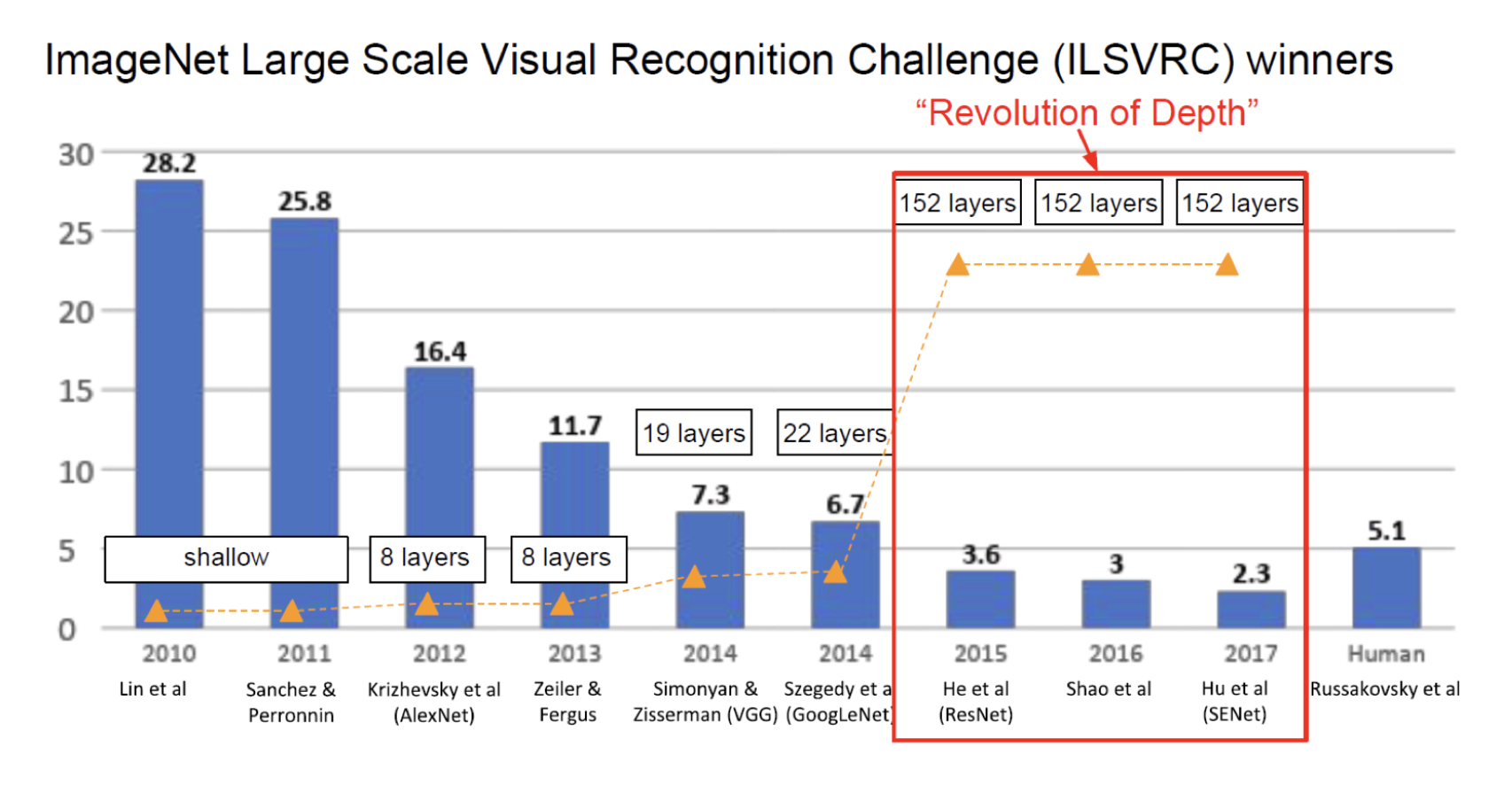
CNN을 연구하면서 기존 모델들은 Layer를 깊게 쌓을수록 성능이 좋아질 것이라고 예상했지만 실제로는 20층 이상의 깊이로 갈 수록 오히려 성능이 떨어지는 현상이 존재하였습니다.

그래서 깊이가 깊어질수록 성능이 좋게 만들 수 있는 방법이 없을까해서 나온 방법이 바로 Resnet이라는 방법입니다.

사진과 같이 152층이라는 엄청나게 깊은 네트워크로 사람의 한계를 뛰어넘은 모습을 볼 수 있습니다.

하지만 이렇게 매우 깊은 네트워크에는 문제점이 존재합니다.

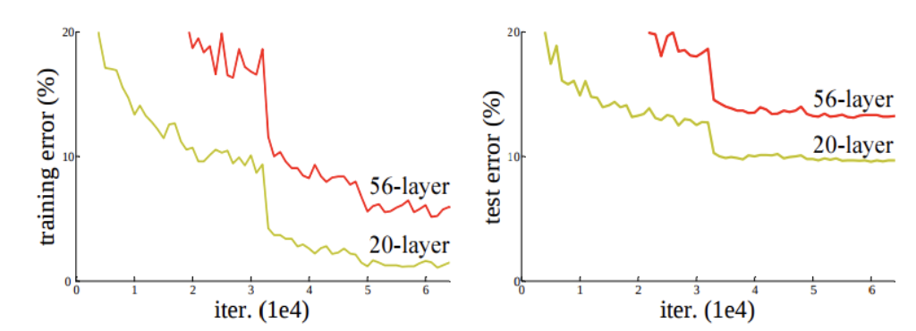
층이 깊어질수록 성능이 떨어지는 것을 보고 직관적으로 Gradient Vanishing/Explosion 이 발생할 수 있음을 짐작할 수 있고, 또한 Degradation 이라는 층이 깊어지면 오히려 성능이 안좋아지는 현상이 발생함을 알 수 있습니다.

이러한 현상의 해결책으로 optimizer함수를 새로 만들어보고자하는 의견이 있었지만, 새로운 optimizer를 만드는 것은 매우 어렵기 때문에, 새로운 Network를 만들기 시작하게 됩니다.

Residual Block

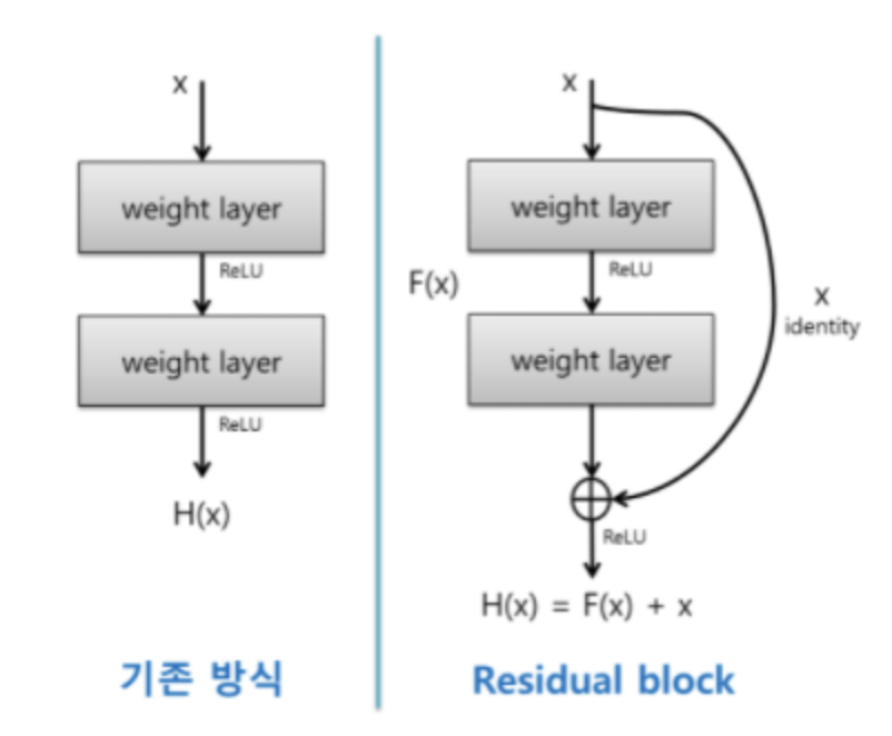
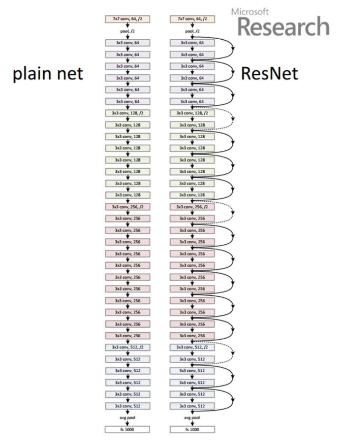
기존 네트워크 방식이 $H(x)$ 일 때, 스킵연결을 만들어서 $x$가 더해지는 방식이 residual block 이고 이를 Skip Connection 이라고 합니다.

우리는 F(x)가 최소가 되는 방향이 목표입니다.

기존 신경망은 $H(x)$가 정답 $y$에 정확히 맵핑이 되는 함수를 찾는 것을 목표로 학습시켜왔던 것이였으므로 기존신경망 $H(x) - x = 0$ 을 만들려 했다면, Resnet은 $H(x)-x=F(x)$로 두어서 $H(x)=x$가 되는 것을 목표로 합니다.

그래서 이러한 main path 에 skip connection이 연결되는 short cut이 생기게 됩니다.

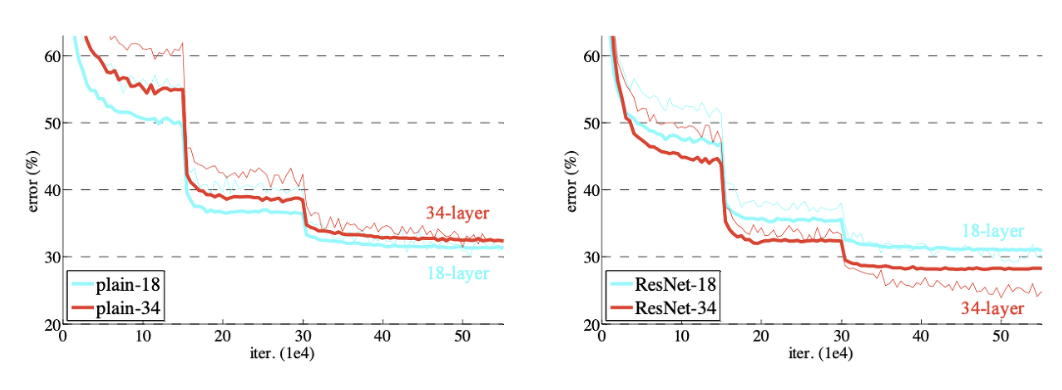
결과적으로 Layer가 깊게 쌓여도 에러가 낮고, degradation problem이 발생하지 않는 것을 볼 수 있습니다.

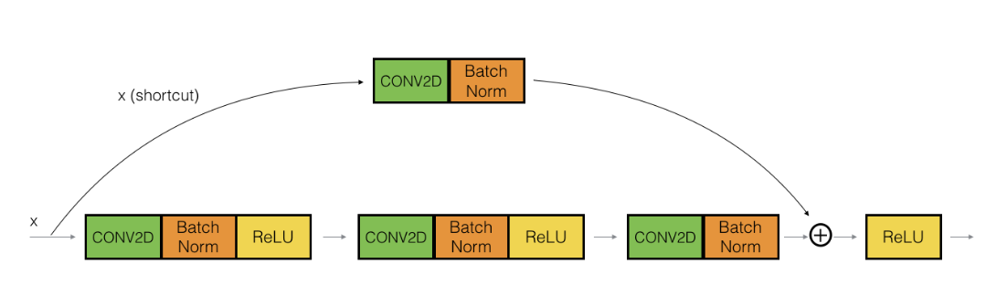
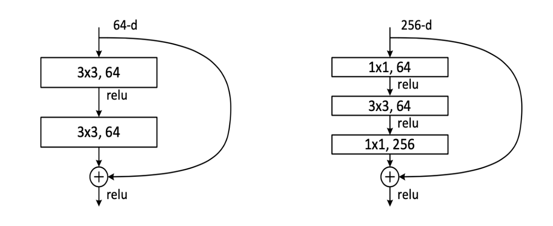
Deeper Bottleneck Architecture

50층 이상의 깊은 모델을 사용할 때는 연산상의 이점을 위해 “bottleneck” layer (1X1 Convolution)을 이용합니다.

사진에서 왼쪽이 Basic Block이고, 오른쪽 그림이 Bottleneck입니다.

1X1 Convolution

1 by 1 convolution의 장점은 크게 다음과 같습니다.

1. Channel 수 조절
2. 연산량 감소
3. 비선형성

1. Channel 수 조절

채널 수는 우리가 원하는만큼 결정할 수 있습니다. 기존의 합성곱연산에서 채널수가 너무 많게 되면 파라미터 수가 급격히 증가하기 때문에 문제가 생기게 됩니다.

하지만 1X1 Convolution을 사용하면 효율적으로 모델으 구성함과 동시에 만족할만한 성능을 얻을 수 있습니다.

파라미터 수가 급격하게 증가하는 것을 예방하기 때문에, Channel 수를 마음껏 조절할 수 있고, 다양한 크기를 가진 합성곱층을 통해 우리가 원하는 구조의 모델을 구성해볼 수 있습니다.

2. 계산량 감소

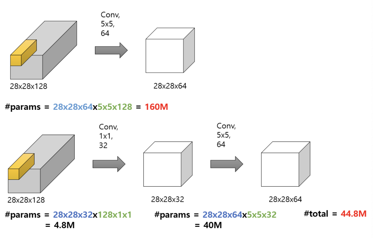
윗 부분은 1억6천만개의 파라미터 수가 필요하고, 아랏 부분은 4백4십만개가 필요하니 약 4배나 차이나는 것을 보실 수 있습니다.

3. 비선형성

1X1 Conv를 사용할 때마다 ReLU 함수도 사용을 하게되는데, ReLU 함수를 사용하는 목적 중 하나는 비선형성을 증가시켜줌이 있습니다.

그러므로 1X1 Conv 를 많이 사용할 수록 랠루함수도 많이 사용을하게 되고, 그 말은 즉, 비선형성이 증가하므로 더 복잡한 패턴도 잘 인식할 수 있게 된다는 의미가 됩니다.

Resnet code 구현

pip install torch-summary

모델의 개요를 확인 할 수 있는 summary가 없어서 다운로드했습니다.

# model
import torch
import torch.nn as nn
import torch.nn.functional as F
from torchsummary import summary
from torch import optim
from torch.optim.lr_scheduler import StepLR

# dataset and transformation
from torchvision import datasets
import torchvision.transforms as transforms
from torch.utils.data import DataLoader
import os

# display images
from torchvision import utils
import matplotlib.pyplot as plt
%matplotlib inline

# utils
import numpy as np
from torchsummary import summary
import time
import copy

기본설정들을 import 해줍니다.

# specify the data path
path2data = 'Anaconda/'

# if not exists the path, make the directory
if not os.path.exists(path2data):
    os.mkdir(path2data)

# load dataset
train_ds = datasets.STL10(path2data, split='train', download=True, transform=transforms.ToTensor())
val_ds = datasets.STL10(path2data, split='test', download=True, transform=transforms.ToTensor())

print(len(train_ds))
print(len(val_ds))

Files already downloaded and verified Files already downloaded and verified
5000
8000

주피터 노트북환경에서 실행하였기 때문에 파일경로가 anaconda 로 진행하였습니다. MNIST 데이터셋 처럼 이번에는 STL10 데이터셋으로 구현을 해보겠습니다.

STL10 Dataset 이란?

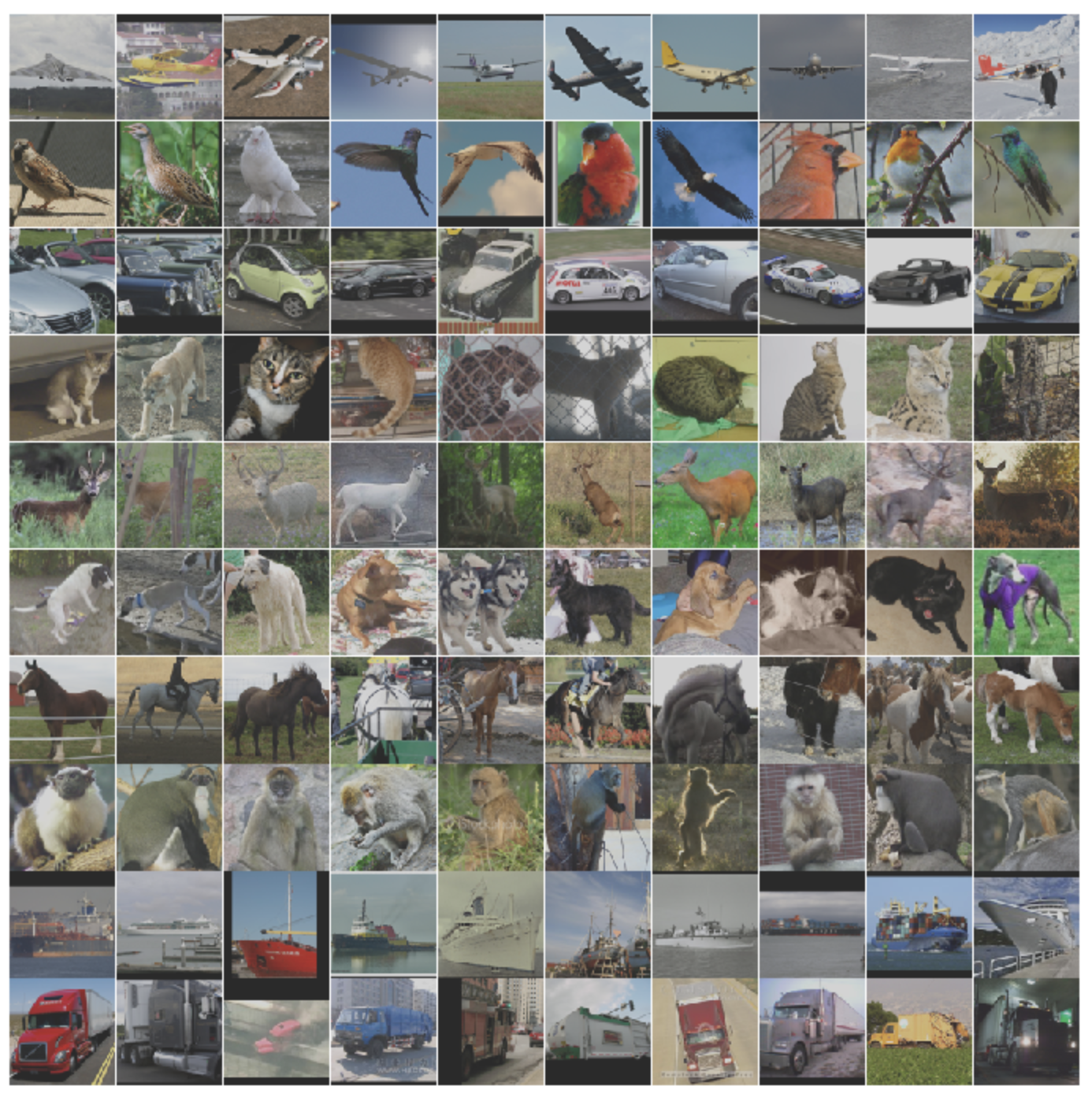
• 10 classes: airplane, bird, car, cat, deer, dog, horse, monkey, ship, truck.
• Images are 96x96 pixels, color.
• 500 training images (10 pre-defined folds), 800 test images per class.
• 100000 unlabeled images for unsupervised learning. These examples are extracted from a similar but broader distribution of images. For instance, it contains other types of animals (bears, rabbits, etc.) and vehicles (trains, buses, etc.) in addition to the ones in the labeled set.

# To normalize the dataset, calculate the mean and std
train_meanRGB = [np.mean(x.numpy(), axis=(1,2)) for x, _ in train_ds]
train_stdRGB = [np.std(x.numpy(), axis=(1,2)) for x, _ in train_ds]

train_meanR = np.mean([m[0] for m in train_meanRGB])
train_meanG = np.mean([m[1] for m in train_meanRGB])
train_meanB = np.mean([m[2] for m in train_meanRGB])
train_stdR = np.mean([s[0] for s in train_stdRGB])
train_stdG = np.mean([s[1] for s in train_stdRGB])
train_stdB = np.mean([s[2] for s in train_stdRGB])


val_meanRGB = [np.mean(x.numpy(), axis=(1,2)) for x, _ in val_ds]
val_stdRGB = [np.std(x.numpy(), axis=(1,2)) for x, _ in val_ds]

val_meanR = np.mean([m[0] for m in val_meanRGB])
val_meanG = np.mean([m[1] for m in val_meanRGB])
val_meanB = np.mean([m[2] for m in val_meanRGB])

val_stdR = np.mean([s[0] for s in val_stdRGB])
val_stdG = np.mean([s[1] for s in val_stdRGB])
val_stdB = np.mean([s[2] for s in val_stdRGB])

print(train_meanR, train_meanG, train_meanB)
print(val_meanR, val_meanG, val_meanB)

0.4467106 0.43980986 0.40664646 0.44723064 0.4396425 0.40495726

데이터셋을 표준화시키기위해서 R, G, B 값에 따라 하나씩 평균값과 표준편차를 구해주는 코드입니다.

# define the image transformation
train_transformation = transforms.Compose([
                        transforms.ToTensor(),
                        transforms.Resize(224),
                        transforms.Normalize([train_meanR, train_meanG, train_meanB],[train_stdR, train_stdG, train_stdB]),
                        transforms.RandomHorizontalFlip(),
])

val_transformation = transforms.Compose([
                        transforms.ToTensor(),
                        transforms.Resize(224),
                        transforms.Normalize([train_meanR, train_meanG, train_meanB],[train_stdR, train_stdG, train_stdB]),
])

이미지파일들을 학습시키기위해 transforms 함수를 통해 텐서로 변환, 사이즈는 224, 그리고 표준화해주는 것을 보실 수가 있습니다.

# apply transforamtion
train_ds.transform = train_transformation
val_ds.transform = val_transformation

# create DataLoader
train_dl = DataLoader(train_ds, batch_size=32, shuffle=True)
val_dl = DataLoader(val_ds, batch_size=32, shuffle=True)

# display sample images 
def show(img, y=None, color=True):
    npimg = img.numpy()
    npimg_tr = np.transpose(npimg, (1,2,0))
    plt.imshow(npimg_tr)

    if y is not None:
        plt.title('labels :' + str(y))

np.random.seed(1)
torch.manual_seed(1)

grid_size = 4
rnd_inds = np.random.randint(0, len(train_ds), grid_size)
print('image indices:',rnd_inds)

x_grid = [train_ds[i][0] for i in rnd_inds]
y_grid = [train_ds[i][1] for i in rnd_inds]

x_grid = utils.make_grid(x_grid, nrow=grid_size, padding=2)

show(x_grid, y_grid)

Clipping input data to the valid range for imshow with RGB data ([0..1] for floats or [0..255] for integers).
image indices: [ 235 3980 905 2763]

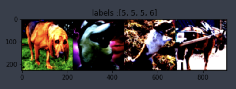
예시 이미지를 출력해보는 코드입니다.

class BasicBlock(nn.Module):
    expansion = 1
    def __init__(self, in_channels, out_channels, stride=1):
        super().__init__()

        # BatchNorm에 bias가 포함되어 있으므로, conv2d는 bias=False로 설정합니다.
        self.residual_function = nn.Sequential(
            nn.Conv2d(in_channels, out_channels, kernel_size=3, stride=stride, padding=1, bias=False),
            nn.BatchNorm2d(out_channels),
            nn.ReLU(),
            nn.Conv2d(out_channels, out_channels * BasicBlock.expansion, kernel_size=3, stride=1, padding=1, bias=False),
            nn.BatchNorm2d(out_channels * BasicBlock.expansion),
        )

        # identity mapping, input과 output의 feature map size, filter 수가 동일한 경우 사용.
        self.shortcut = nn.Sequential()

        self.relu = nn.ReLU()

        # projection mapping using 1x1conv
        if stride != 1 or in_channels != BasicBlock.expansion * out_channels:
            self.shortcut = nn.Sequential(
                nn.Conv2d(in_channels, out_channels * BasicBlock.expansion, kernel_size=1, stride=stride, bias=False),
                nn.BatchNorm2d(out_channels * BasicBlock.expansion)
            )

    def forward(self, x):
        x = self.residual_function(x) + self.shortcut(x)
        x = self.relu(x)
        return x


class BottleNeck(nn.Module):
    expansion = 4
    def __init__(self, in_channels, out_channels, stride=1):
        super().__init__()

        self.residual_function = nn.Sequential(
            nn.Conv2d(in_channels, out_channels, kernel_size=1, stride=1, bias=False),
            nn.BatchNorm2d(out_channels),
            nn.ReLU(),
            nn.Conv2d(out_channels, out_channels, kernel_size=3, stride=stride, padding=1, bias=False),
            nn.BatchNorm2d(out_channels),
            nn.ReLU(),
            nn.Conv2d(out_channels, out_channels * BottleNeck.expansion, kernel_size=1, stride=1, bias=False),
            nn.BatchNorm2d(out_channels * BottleNeck.expansion),
        )

        self.shortcut = nn.Sequential()

        self.relu = nn.ReLU()

        if stride != 1 or in_channels != out_channels * BottleNeck.expansion:
            self.shortcut = nn.Sequential(
                nn.Conv2d(in_channels, out_channels*BottleNeck.expansion, kernel_size=1, stride=stride, bias=False),
                nn.BatchNorm2d(out_channels*BottleNeck.expansion)
            )
            
    def forward(self, x):
        x = self.residual_function(x) + self.shortcut(x)
        x = self.relu(x)
        return x

class ResNet(nn.Module):
    def __init__(self, block, num_block, num_classes=10, init_weights=True):
        super().__init__()

        self.in_channels=64

        self.conv1 = nn.Sequential(
            nn.Conv2d(3, 64, kernel_size=7, stride=2, padding=3, bias=False),
            nn.BatchNorm2d(64),
            nn.ReLU(),
            nn.MaxPool2d(kernel_size=3, stride=2, padding=1)
        )

        self.conv2_x = self._make_layer(block, 64, num_block[0], 1)
        self.conv3_x = self._make_layer(block, 128, num_block[1], 2)
        self.conv4_x = self._make_layer(block, 256, num_block[2], 2)
        self.conv5_x = self._make_layer(block, 512, num_block[3], 2)

        self.avg_pool = nn.AdaptiveAvgPool2d((1,1))
        self.fc = nn.Linear(512 * block.expansion, num_classes)

        # weights inittialization
        if init_weights:
            self._initialize_weights()

    def _make_layer(self, block, out_channels, num_blocks, stride):
        strides = [stride] + [1] * (num_blocks - 1)
        layers = []
        for stride in strides:
            layers.append(block(self.in_channels, out_channels, stride))
            self.in_channels = out_channels * block.expansion

        return nn.Sequential(*layers)

    def forward(self,x):
        output = self.conv1(x)
        output = self.conv2_x(output)
        x = self.conv3_x(output)
        x = self.conv4_x(x)
        x = self.conv5_x(x)
        x = self.avg_pool(x)
        x = x.view(x.size(0), -1)
        x = self.fc(x)
        return x

    # define weight initialization function
    def _initialize_weights(self):
        for m in self.modules():
            if isinstance(m, nn.Conv2d):
                nn.init.kaiming_normal_(m.weight, mode='fan_out', nonlinearity='relu')
                if m.bias is not None:
                    nn.init.constant_(m.bias, 0)
            elif isinstance(m, nn.BatchNorm2d):
                nn.init.constant_(m.weight, 1)
                nn.init.constant_(m.bias, 0)
            elif isinstance(m, nn.Linear):
                nn.init.normal_(m.weight, 0, 0.01)
                nn.init.constant_(m.bias, 0)

def resnet18():
    return ResNet(BasicBlock, [2,2,2,2])

def resnet34():
    return ResNet(BasicBlock, [3, 4, 6, 3])

def resnet50():
    return ResNet(BottleNeck, [3,4,6,3])

def resnet101():
    return ResNet(BottleNeck, [3, 4, 23, 3])

def resnet152():
    return ResNet(BottleNeck, [3, 8, 36, 3])

device = torch.device('cuda' if torch.cuda.is_available() else 'cpu')
model = resnet50().to(device)
x = torch.randn(3, 3, 224, 224).to(device)
output = model(x)
print(output.size())

torch.Size([3, 10])

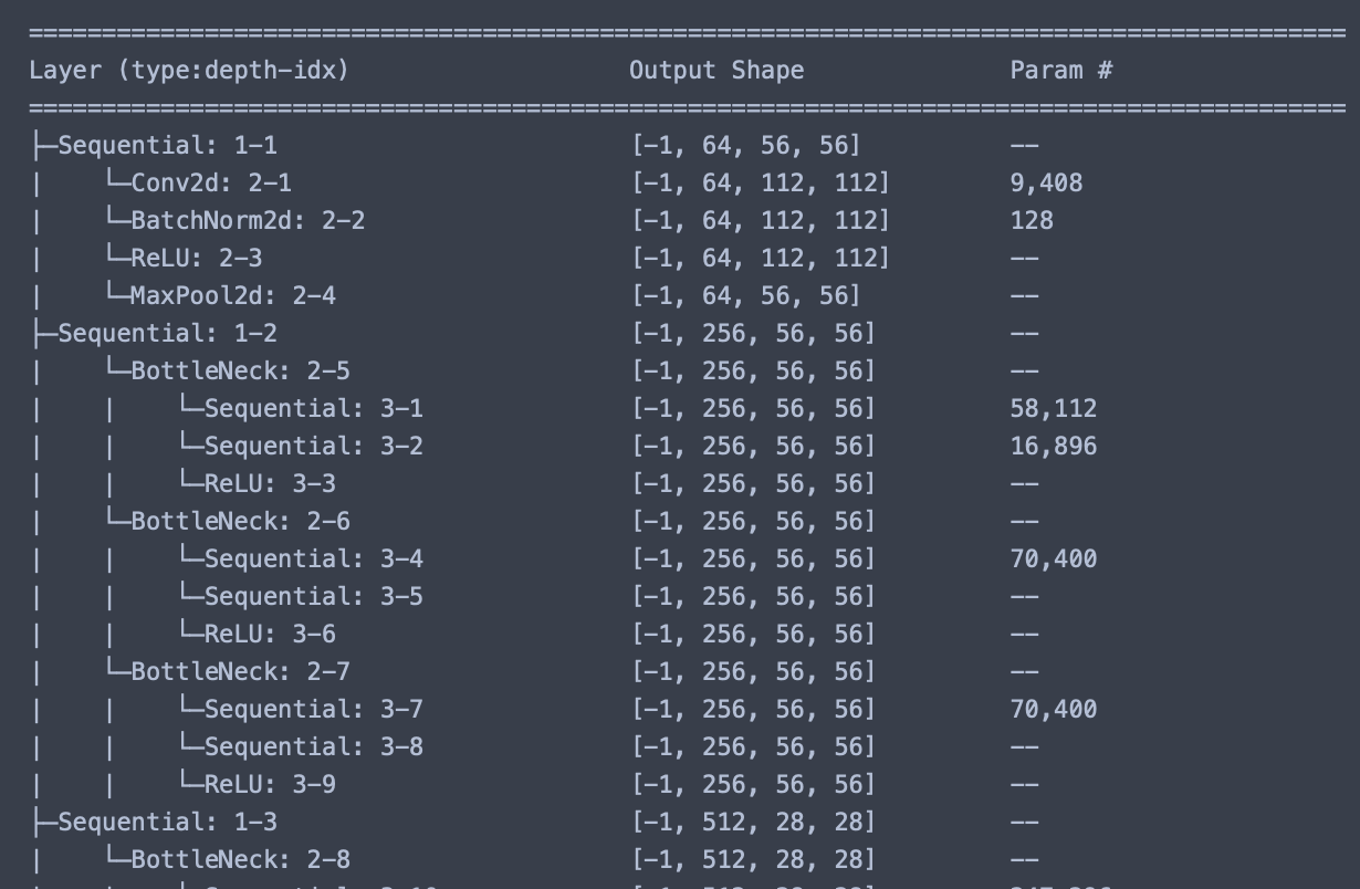
이제 여기서 summary함수를 이용해 전체적인 구조를 살펴보겠습니다. 워낙에 내용이 길기 때문에 앞부분만 캡쳐해보겠습니다, 궁금하신분들은 직접 해보셔도 좋을 것 같습니다.

summary(model, (3, 224, 224), device=device.type)

loss_func = nn.CrossEntropyLoss(reduction='sum')
opt = optim.Adam(model.parameters(), lr=0.001)

from torch.optim.lr_scheduler import ReduceLROnPlateau
lr_scheduler = ReduceLROnPlateau(opt, mode='min', factor=0.1, patience=10)

손실 함수와 옵티마이저 그리고 학습률 스케쥴러를 정의해줍니다.

# function to get current lr
def get_lr(opt):
    for param_group in opt.param_groups:
        return param_group['lr']

현재 lr을 계산하는 함수라고 합니다.

# function to calculate metric per mini-batch
def metric_batch(output, target):
    pred = output.argmax(1, keepdim=True)
    corrects = pred.eq(target.view_as(pred)).sum().item()
    return corrects


# function to calculate loss per mini-batch
def loss_batch(loss_func, output, target, opt=None):
    loss = loss_func(output, target)
    metric_b = metric_batch(output, target)

    if opt is not None:
        opt.zero_grad()
        loss.backward()
        opt.step()

    return loss.item(), metric_b

배치당 loss 와 metric을 계산하는 함수입니다.

# function to calculate loss and metric per epoch
def loss_epoch(model, loss_func, dataset_dl, sanity_check=False, opt=None):
    running_loss = 0.0
    running_metric = 0.0
    len_data = len(dataset_dl.dataset)

    for xb, yb in dataset_dl:
        xb = xb.to(device)
        yb = yb.to(device)
        output = model(xb)

        loss_b, metric_b = loss_batch(loss_func, output, yb, opt)

        running_loss += loss_b
        
        if metric_b is not None:
            running_metric += metric_b
        
        if sanity_check is True:
            break

    loss = running_loss / len_data
    metric = running_metric / len_data

    return loss, metric

epoch 당 loss를 정의하는 함수입니다.

# function to start training
def train_val(model, params):
    num_epochs=params['num_epochs']
    loss_func=params["loss_func"]
    opt=params["optimizer"]
    train_dl=params["train_dl"]
    val_dl=params["val_dl"]
    sanity_check=params["sanity_check"]
    lr_scheduler=params["lr_scheduler"]
    path2weights=params["path2weights"]

    loss_history = {'train': [], 'val': []}
    metric_history = {'train': [], 'val': []}

    best_loss = float('inf')

    start_time = time.time()

    for epoch in range(num_epochs):
        current_lr = get_lr(opt)
        print('Epoch {}/{}, current lr={}'.format(epoch, num_epochs-1, current_lr))

        model.train()
        train_loss, train_metric = loss_epoch(model, loss_func, train_dl, sanity_check, opt)
        loss_history['train'].append(train_loss)
        metric_history['train'].append(train_metric)

        model.eval()
        with torch.no_grad():
            val_loss, val_metric = loss_epoch(model, loss_func, val_dl, sanity_check)
        loss_history['val'].append(val_loss)
        metric_history['val'].append(val_metric)

        if val_loss < best_loss:
            best_loss = val_loss
            # best_model_wts = copy.deepcopy(model.state_dict())

            # torch.save(model.state_dict(), path2weights)
            # print('Copied best model weights!')
            print('Get best val_loss')

        lr_scheduler.step(val_loss)

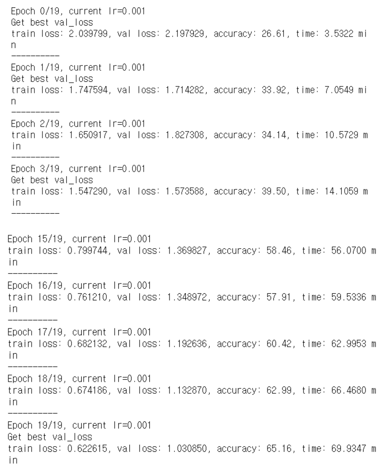
        print('train loss: %.6f, val loss: %.6f, accuracy: %.2f, time: %.4f min' %(train_loss, val_loss, 100*val_metric, (time.time()-start_time)/60))
        print('-'*10)

    # model.load_state_dict(best_model_wts)

    return model, loss_history, metric_history

# definc the training parameters
params_train = {
    'num_epochs':20,
    'optimizer':opt,
    'loss_func':loss_func,
    'train_dl':train_dl,
    'val_dl':val_dl,
    'sanity_check':False,
    'lr_scheduler':lr_scheduler,
    'path2weights':'./models/weights.pt',
}

# create the directory that stores weights.pt
def createFolder(directory):
    try:
        if not os.path.exists(directory):
            os.makedirs(directory)
    except OSerror:
        print('Error')
createFolder('./models')

하이퍼파라미터를 정의합니다.

model, loss_hist, metric_hist = train_val(model, params_train)

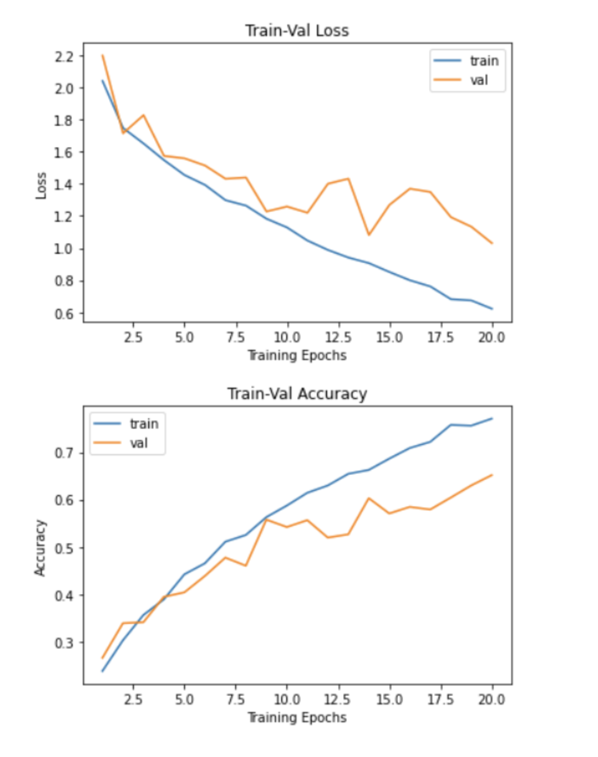
# Train-Validation Progress
num_epochs=params_train["num_epochs"]

# plot loss progress
plt.title("Train-Val Loss")
plt.plot(range(1,num_epochs+1),loss_hist["train"],label="train")
plt.plot(range(1,num_epochs+1),loss_hist["val"],label="val")
plt.ylabel("Loss")
plt.xlabel("Training Epochs")
plt.legend()
plt.show()

# plot accuracy progress
plt.title("Train-Val Accuracy")
plt.plot(range(1,num_epochs+1),metric_hist["train"],label="train")
plt.plot(range(1,num_epochs+1),metric_hist["val"],label="val")
plt.ylabel("Accuracy")
plt.xlabel("Training Epochs")
plt.legend()
plt.show()

아직 완전 세세하게 코드들이 이해가 가지는 않아서 ㅜㅜ 더 공부해봐야 할 것 같네요,,,

참고문헌

끝!